
One of the most prominent challenges posed in discretionary trading is not the lack of information, or access to it, but rather distinguishing the signal from the noise, deciding which information deserves to change our interpretation.
This article takes a top-down approach to three practical questions:
- Where has the market conducted meaningful business, and how did it resolve?
- Which decisions remain unresolved?
- What lower timeframe activity supports or rejects the thesis?
Through Auction Market Theory (AMT), ATAS’s analytical tools, and a real trading session involving Gold and Silver, we will examine how to move from a structured hypothesis to conditional execution. It also shows how to set up ATAS for this auction market theory trading workflow.
- Auction market theory (AMT) trading starts with location: volume profile nodes and market-generated reference levels show where participants must make decisions.
- High volume nodes mark accepted prices; low volume nodes mark imbalanced prices that are crossed quickly, rejected, or turned into new acceptance.
- Volume and Delta measure effort; price response shows whether that effort produced a result.
- The top-down framework has four steps: establish what the higher timeframe has decided, define what remains unresolved, build if-then scenarios, and test them on the lower timeframe.
- In the September 25, 2026 Gold session, the same volume node first supported a conditional long and, once it was lost, a re-offer.
Auction Market Theory Basics: Why Location Matters
Auction Market Theory (AMT) treats a market as a continuous two-way auction whose purpose is to facilitate trade. Price moves to find levels where buyers and sellers will transact, rotates while both sides remain willing, and extends when one side can no longer be accommodated. ATAS’s article The Auction Market Theory covers the broader background.
Location comes first because the same activity means different things in different places. A response at the edge of an earlier auction tests a decision participants have already made. The same response in the middle of a range usually carries less weight.
Start now!
Try ATAS free with no time limit
Balance vs Imbalance: How Markets Search for Acceptance
Markets are in an unbounded process of discovery, but can only be in one of two states: balance or imbalance. In a balanced auction, substantial two-way business occurs across an established range, and trade keeps returning toward a familiar distribution. In an imbalanced auction, price extends away from a given distribution to test whether business can develop elsewhere. Neither condition is permanent.
Consider a market that violently breaks a prior low, then immediately regains the preceding range. The break is observable, but the more important information is that selling failed to sustain those lower prices. In combination, those observations may weaken a continuation thesis, and yet they do not guarantee a reversal either.
Video 1 | Balance vs imbalance. Educational schematic. The schematic shows a range building two-way trade, a breakout testing new prices, and the auction either accepting the new area or returning to prior value.
Why Not Every Price Move Is Tradable
A market can move substantially without providing a useful location from which to establish a hypothesis or frame risk. A strong upward candle in the middle of a balance says little about the room to the next reference. A smaller response after a failed attempt to auction below the prior week’s low says more, because an earlier directional attempt is being tested.
This is why I begin with location rather than an entry pattern. I want to recognize areas where participants will be forced to make a decision about their existing inventory (the positions they already hold), and where new activity can test the consequences of earlier business.
How to Find Key Levels with Volume Profile
A volume profile (VP) is a tool that organizes executed transactions by price, rather than by time. It enables us to examine where business concentrated, where comparatively little activity occurred, and how those distributions developed over time. Figure 1 shows Gold’s August 2026 monthly profile on the daily chart:
- Point of Control (POC): the price with the most volume in the selected period, the yellow line near 4,450.
- High volume node (HVN): a wide part of the profile, approximately 4,405 to 4,485 around August’s main POC, with a second near 4,640 to 4,705.
- Low volume node (LVN): a narrow section between distributions, here roughly 4,560 to 4,630.
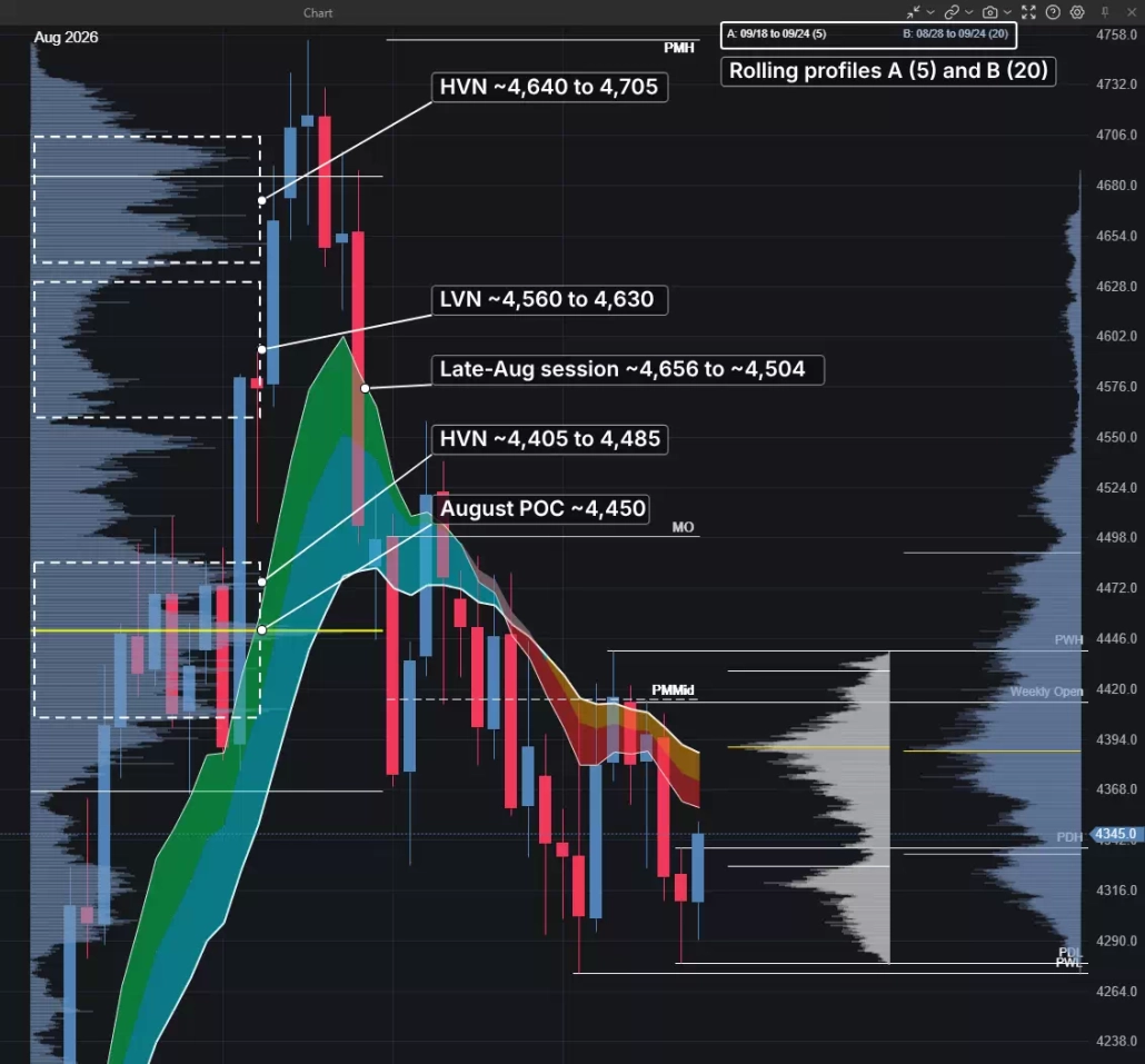
Figure 1 | Gold daily, September 25, 2026, 08:28 ET. August profile: POC near 4,450; HVNs approximately 4,405 to 4,485 and 4,640 to 4,705; LVN approximately 4,560 to 4,630. Zone boundaries are interpretive.
High Volume Nodes: Where the Market Accepted Price
A high volume node (HVN) represents an area of balance, where there is a concentration of completed transactions within a given price range. The market spent time trading there, creating a recognizable area of established trade, known as ‘acceptance’. The node becomes especially relevant once price expands away from it.
Gold built August’s main node before rallying above 4,700, so the node became a structural reference. On a return, I watch for a rebid (buyers returning to the area) or for selling to trade through the resting bids and build value below, which would leave earlier buying offside, meaning positioned against the current price. The historical node locates the test, and the current response decides whether it still matters.
The Point of Control (POC) identifies the price at which the greatest volume was executed over a selected period. A migrating POC shows where completed business is shifting, without independently establishing directional control.
Low Volume Nodes: Where the Market Rejected Price
A low volume node (LVN) is an area where comparatively little business was completed, and therefore represents an area of price where the auction was heavily imbalanced. These pockets develop between established distributions when price is moving directionally through a range without developing sustained two-way trade. When price returns to these levels, three outcomes can be told apart:
- Efficient traversal: price moves through quickly, with little new volume, toward the next distribution. In late August one session carried Gold from about 4,656 to about 4,504 through the LVN in Figure 1.
- Rejection: the probe makes limited progress and price returns toward the distribution it came from, or ignites the next leg of imbalance through the other end.
- New acceptance: trade slows and fresh volume builds inside the thin area, turning it into a node: a new willingness to transact in a previously imbalanced price area.
Video 2 | Volume Profile, HVNs and LVNs. Educational schematic. It shows how a profile forms wide high volume nodes and thin low volume nodes, and the three ways price can behave when it returns to a thin area.
Reference Levels: Prior Week/Day Highs and Lows, Opens, Initial Balance, Range Edges
Market-Generated Information (MGI) is the set of reference prices the auction itself creates. MGIs include anything from:
- Prior day high/low (PDH/PDL) and Globex prior day high/low (GPDH/GPDL): the preceding session’s extremes. Here, intraday PDH/PDL use regular trading hours (RTH); GPDH/GPDL include overnight trade. Daily-chart values cover the full session.
- Prior week and month (PWH, PWL, PMH, PML, PMMid): high, low and midpoint of the higher timeframe auctions.
- Opens: weekly open (WO, the first trade of the Sunday 18:00 session), monthly open (MO), regular-trading-hours session open (Open) and New York open (NYO).
- Initial balance (IB H/L/Mid) and opening range (OR H/L/Mid): the high, low and midpoint of defined opening windows. The initial balance usually covers the first hour; shorter opening ranges and extensions such as OR −0.5x use the chosen window’s height.
With this context, the chart becomes a map of where decisions are due. A reference itself does not determine an opportunity. Its value comes from how the market interacts with it.
Setting Up ATAS for Auction Market Theory Trading
My workspace is organized around four complementary views of the same auction, moving from what the market has already accomplished, to locations where new activity can test that interpretation, to the order flow at those inflections. Each chart answers a different question.
Data, session and time (as displayed in the September 25th captures):
- Gold: #GCZ6 (Continuous(GC)).
- Silver: #SILZ6 (Continuous(SIL)).
- Session: ETH, selected at the bottom of each chart, the CME Globex day from 18:00 to 17:00, so each daily bar includes the prior evening.
- Time: chart times are US Eastern, and all times here are ET.
The four views:
- Daily (Figure 1). Period D, with five- and twenty-session rolling profiles (A and B; on September 25 they covered September 18 to 24 and August 28 to September 24) and calendar-based monthly profiles.
- One-hour (Figure 6, in the case study). Period H1. Each session carries its own full-session profile, POC in yellow and value area edges dashed; the right-sided H VAH, H POC and H VAL belong to the five-session rolling volume profile.
- Five-minute footprint (Figure 7a). Period M5, with the native Delta indicator below. Its legend in the captures reads Delta (Bars, 0.0, True), which I read as bar display with no filter. Native Delta resets with each bar; it does not accumulate like Cumulative Delta.
- 150-contract volume chart. Period 150V, the Volume 150 preset in the period list (Figure 2). Each bar closes after 150 Gold contracts trade, regardless of time; 150 is how the bars are built, not an order size. This is my execution chart, carrying the RTH profile, the leg to leg delta profile and the Delta heatmap.
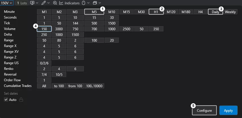
Figure 2 | ATAS period list, 1 M5, 2 H1, 3 Daily, 4 Volume 150 (150V), 5 Configure.
Footprint settings (Figure 3). Open the chart’s Settings, then Footprint settings. In the current workspace, Content is Volume, Mode is Volume profile and Color scheme is Heatmap by volume; Show Text is on, the values divider is 1, the value area is shaded, Bid/Ask Imbalance is disabled and no filters are set. Choose the content that answers your question rather than copying a palette.
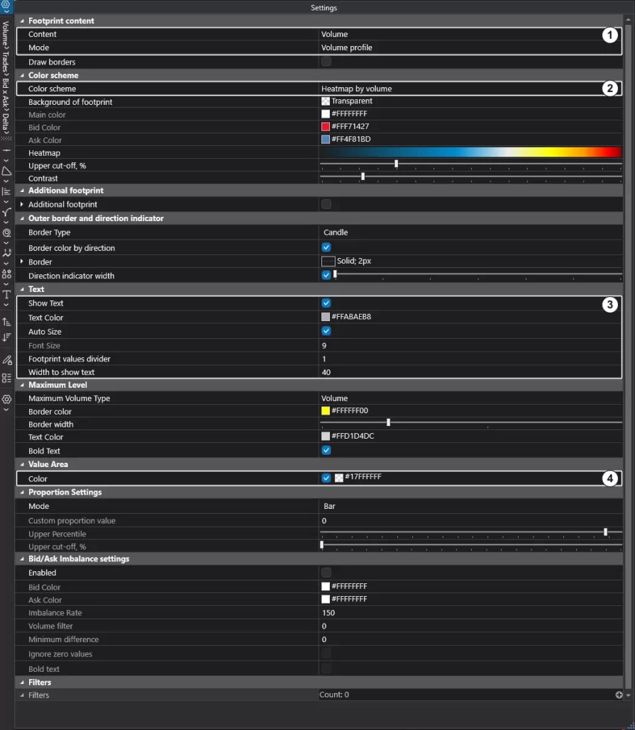
Figure 3 | Footprint settings, 1 Content and Mode, 2 Color scheme, 3 Text, 4 Value area.
Profiles (Figure 4). Profiles A and B come from a custom study, ETV Rolling Session Profile, currently set to an 18:00 to 17:00 session, 20 and 5 sessions, 2 ticks per row and a 70 percent value area. The monthly profiles come from ETV Monthly Volume Profile (currently 12 months, 4 ticks per row, 70 percent value area).
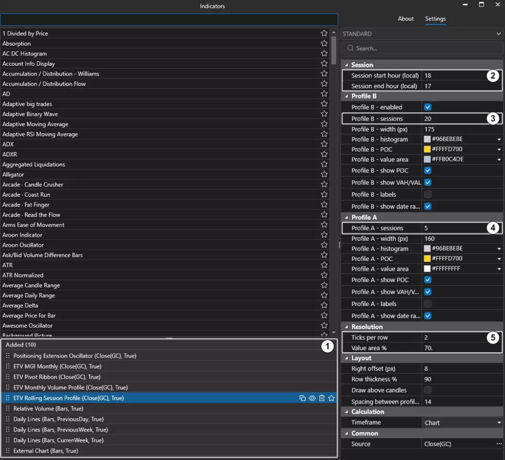
Figure 4 | ETV Rolling Session Profile (custom) settings, 1 studies on the chart, 2 session hours, 3 Profile B, 4 Profile A, 5 resolution and value area.
What the custom studies do. Several studies on my charts are customized rather than native. Each answers one question faster than I could by hand; none is required, and most have a native or manual route.
| Study | What it shows | Native ATAS route |
|---|---|---|
| Reference levels (ETV MGI) | Draws the levels listed above on every intraday chart, so I am not redrawing the map each session. | Use native Daily Lines where supported, or Horizontal Line drawings at the selected session’s high, low or open. |
| Rolling and monthly profiles (ETV Rolling Session Profile, ETV Monthly Volume Profile; Figure 4) | Profile A covers the last 5 sessions and B the last 20, so the week’s value (H VAH, H POC, H VAL) rolls forward daily instead of resetting on Monday; the monthly profile keeps completed months such as August’s node in Figure 1. | For five or twenty sessions, select Fixed Volume Profile & TPO from the drawing toolbar’s Volume analysis group. Set Mode to Profile and Profile type to Volume, then draw across the completed sessions. Advance the window manually after each close. For calendar months, use the Volume Profile & TPO indicator in Profile mode with External Period set to Monthly. |
| Pivot ribbon (ETV EMA Pivot Ribbon Band; Figures 5 and 7a) | A band of exponential moving averages showing the slope on the timeframe that frames the trade and the one that executes it. On September 25 it sloped down above price on both, so the long was taken against the prevailing slope and needed the order flow to confirm it. | Utilize a set of two or more EMA indicators. |
| RTH volume profile (Figures 8 and 10) | Volume by price for the day session only, so overnight trade does not blur where the day is building value. | Volume Profile & TPO on a custom period starting at the day-session open. |
| Leg to leg delta profile and Delta heatmap (Figures 8, 10 and 11) | The profile prints Delta by price for the latest swing legs, and the heatmap colors each 150V bar by its Delta, so I can see where and when aggression printed within a leg. That is how I locate the last offside participants and set my stop just beyond their orders (Step 4). | Set the footprint’s Content to Delta and read Delta by price across the bars of the leg. |
The purpose of this arrangement is not to display the greatest quantity of information. It is to isolate the few variables that contribute meaningfully to my interpretation of the auction.
Reading Order Flow at the Level: Delta, Volume and Price Response
A meaningful location gives the hypothesis a reference, not an entry. On the five-minute and volume charts, I test the thesis by separating three observations: how much business was completed and where, who demanded immediacy, and what price accomplished as a result.
Volume measures executed participation. Delta is volume executed at the ask minus volume executed at the bid, so it shows which side initiated. Neither metric shows the inventory yet to be filled or the intent behind an order; it is the market’s response that turns these neutral observations into actionable choices.
Effort vs Result: Does Aggression Move Price?
Suppose Gold reaches the upper edge of a distribution with strong positive Delta. If price sustains trade beyond the reference and holds a retest, the initiative coincided with discovery. If buyers stay aggressive while progress stalls, the same Delta represents ineffective initiative.
Market orders consume liquidity resting passively on the order book. Significant aggressive activity can therefore encounter sufficient opposing interest to prevent meaningful progress.
Think of someone running full force into a door that someone larger is holding shut: the effort is substantial, but the result is limited. What matters is the proportion between effort and progress, not the size of the aggression in isolation.
When Aggression Fails to Produce Price Discovery
A positive feedback loop develops when activity reinforces price’s direction: aggressive buyers consume the resting offers, sellers pull liquidity and offer higher, and later buyers must pay up. If that pressure persists, the market feeds on its own momentum.
A negative feedback loop develops when the move finds counterparties that match or overpower it. As price advances, additional sellers become willing to transact, while earlier buyers grow vulnerable or become unwilling to pay higher prices.
In ATAS, the negative loop looks like a large Delta bar and heavy footprint prints on a bar that fails to extend: at 09:00 (Figure 7a, Delta near −96) and at 09:35 (Figure 9, Delta near +118). On the 150V chart, the leg to leg delta profile shows it by price, as large cells that price leaves behind rather than extends from (Figures 8 and 10). Video 3 illustrates the loop schematically.
When executing, I want to lean against aggressive activity that is going unrewarded, or participate with activity that keeps producing meaningful progress.
Video 3 | Order Flow and feedback. Educational schematic. It shows aggression either feeding a positive loop that extends price, or meeting opposing liquidity and stalling in a negative loop.
AMT Trading Example: Top-Down Analysis of Gold and Silver Futures in ATAS
The following sequence comes from Friday, September 25, 2026. Gold was the principal execution instrument. Silver served as a background structural check, rather than an independent entry signal. It includes an initial conditional long, its failure, and a re-offer (a short from the level the bid had lost).
Step 1. What Has the Higher Timeframe Already Decided?
First, I establish what participants have already accomplished and where they will be forced to make decisions about existing inventory.
- Sunday evening to Tuesday: the week opened at 4,413.0 (D1). Monday and Tuesday traded above it but could not hold (D2). Tuesday rejected a probe to about 4,328, closed near 4,396 and built a node from about 4,350 to 4,374, with its POC at 4,373.9 (D3).
- Wednesday: the session failed from about 4,408, liquidated through Tuesday’s node and closed near 4,323, leaving the week’s earlier buying offside (D4).
- Thursday: selling pressed below Wednesday’s low of 4,311.0 to 4,278.2, into the thin lower tail of the five-session profile, but could not hold and closed near 4,310 (D5).
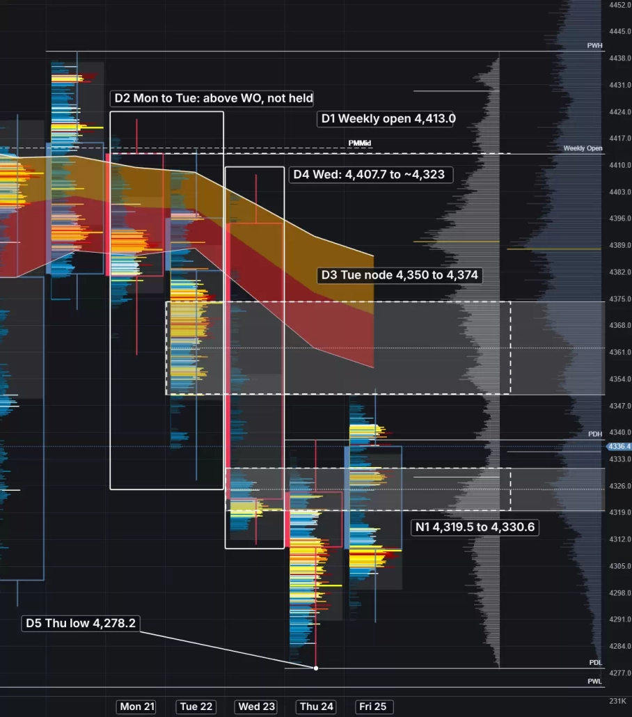
Figure 5 | Gold daily footprint, September 25, 08:38 ET (Friday’s bar still forming). D1 to D5 mark the week’s decisions; N1 is the lower node.
Thursday’s value had shifted lower, but without sustained downside progress. This was my first observation: the effort higher had failed on Wednesday, and the effort lower had grown ineffective on Thursday, potentially leaving the latest selling vulnerable.
Step 2. What Remains Unresolved Overnight and Pre-Market?
Overnight, Gold held above Thursday’s low, at about 4,290, then recovered through the lower node and above the prior day high of 4,338. That node, about 4,320 to 4,331 (N1 in Figure 6), was where Wednesday’s liquidation ended, holding Wednesday’s POC and the five-session value area low (H VAL, 4,323.6). Thursday’s selling had started inside it and was now offside. Overhead sat Tuesday’s node (about 4,350 to 4,374); the pre-market high, near 4,352, stalled at its lower edge.
I could therefore frame the agenda around one unresolved question: could the bid accumulate against the recaptured lower node and continue to develop value above it, or would that recovery fail and restore the downward auction?
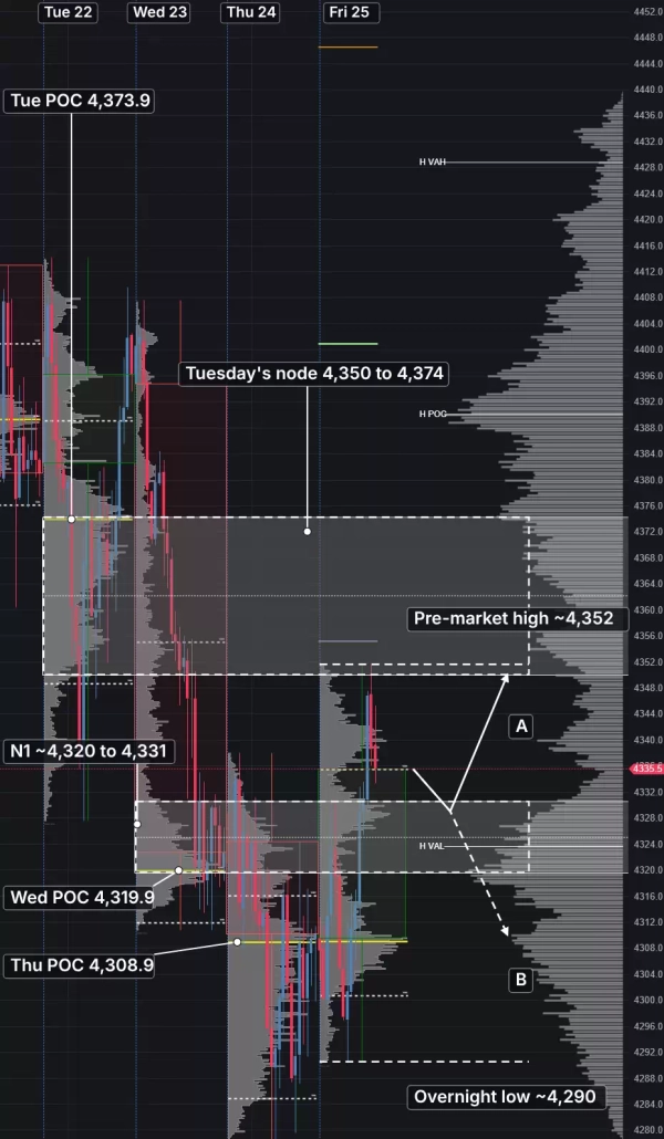
Figure 6 | Gold one-hour, September 25, 08:37 ET. N1, Tuesday’s node, session POCs and the overnight range, with scenarios A and B.
Step 3. Building If-Then Scenarios
Before the session begins, I set three conditional scenarios; A and B are marked on Figure 6.
Scenario A, rebid. If Gold revisited N1 just inside the five-day dealing range, selling failed to extend and buyers began building inventory higher, the long thesis would have material evidence behind it. The pre-market high near 4,352, at the lower edge of Tuesday’s node, would be the place to reassess progress and begin reducing exposure.
Scenario B, failed recovery. If Gold lost N1, began to build interest below it and the bid could not regain it, the re-offer thesis would strengthen. Scenario C, stay flat. If participants did not respond at N1 as expected, no trade was the appropriate decision.
| Scenario | Condition at N1 | Plan |
|---|---|---|
| A. Rebid | Selling fails to extend and buyers begin building inventory higher | Conditional long; reassess and reduce exposure near the pre-market high (about 4,352) |
| B. Failed recovery | Gold loses N1, builds interest below it, and the bid cannot regain it | Re-offer: short against offside inventory higher |
| C. Stay flat | Participants do not respond at N1 as expected | No trade |
These scenarios make the trade-off between price and information explicit: executing at the first touch improves location with less confirmation, while waiting for a reclaim or failed retest improves the evidence but shortens the runway. There is no such thing as a solution, only trade-offs. I consider this the ticket cost of participating: before committing risk, I want to know which uncertainty I am paying to resolve, and where the thesis becomes invalid.
Step 4. Testing the Scenario on the Lower Timeframe
Figure 7a shows the five-minute footprint at 09:08:33, and Figure 8 the 150V chart at the same moment:
- E1, the 09:00 bar (complete): Gold traded into N1, reaching about 4,326.5, with Delta near −96. Sellers were aggressive, yet price barely extended past the five-minute node’s lower edge at 4,327. The offer got stuffed, meaning its aggression was absorbed without progress.
- E2, the 09:05 bar (still forming): Delta read +99 at the capture and price had returned to about 4,332.7, above the node and the opening range low (4,332.3). The responsive bid, buyers reacting to the test, had turned initiative, pressing price higher.
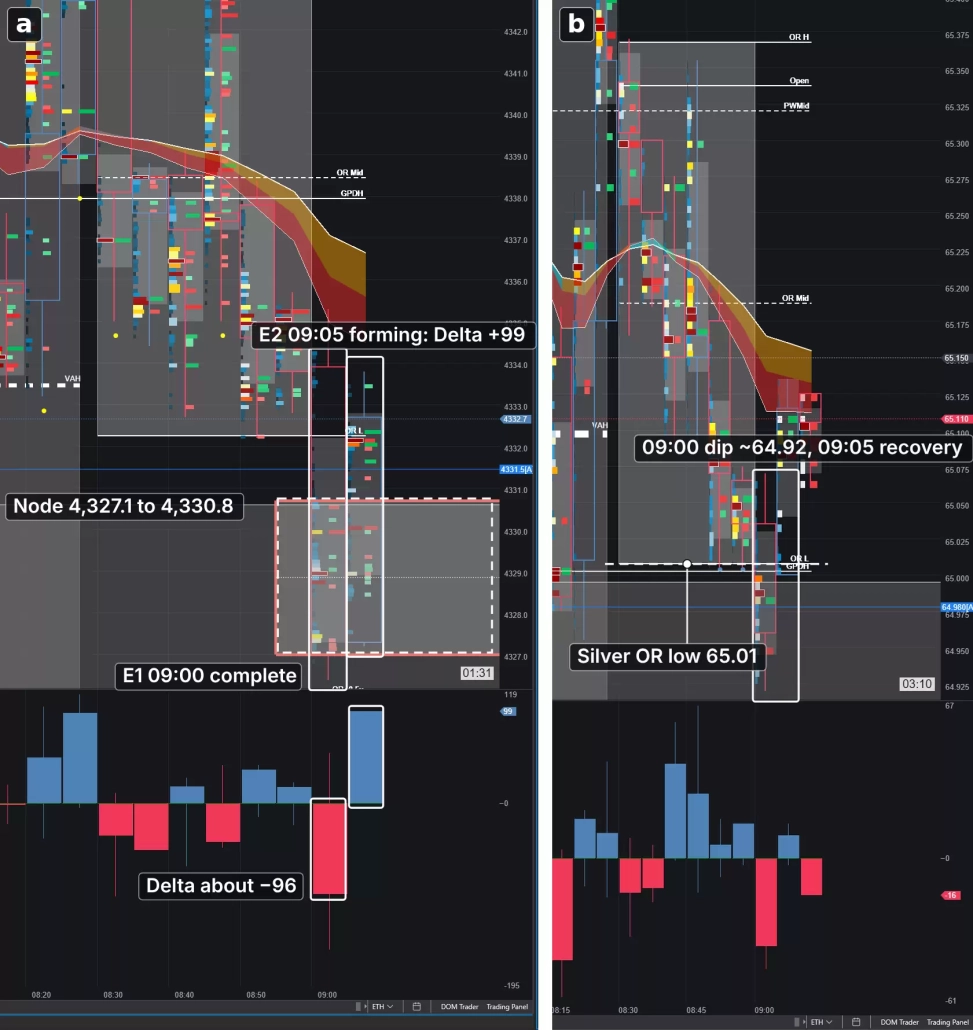
Figure 7 | September 25. (a, left) Gold five-minute footprint, 09:08:33 ET: E1 complete, E2 forming. (b, right) Silver five-minute, 09:11:54 ET: the same dip and recovery.
On the 150V chart, the leg to leg delta profile shows when and where that selling was absorbed: it prints the leg’s sellers at 4,327 to 4,330, while the heatmap colors those bars red and the bar that reclaimed the node blue, back above the RTH value area low (4,331.6). The offer had gone offside at the node.
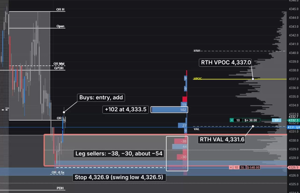
Figure 8 | Gold 150V, September 25, 09:08:33 ET. Leg Delta, RTH volume point of control (VPOC), value area low, buy markers and displayed protective stop. Leg sellers about −38, −30 and −54 at 4,327 to 4,330; +102 at 4,333.5 on the reclaim.
My conditional long was established on that sequence, and I added once as the bid continued to prove itself and push the offer further offside. I set stops just beyond the last offside participants’ orders rather than beyond the price swing itself. Here that meant 4,326.9, at the leg’s last large selling cell (about −54 near 4,327), above the 4,326.5 swing low: if the offer traded back through it, those sellers were onside again and the thesis was wrong.
In this case, the auction did not sustain trade higher. The offer regained control of the area where its aggression had begun, turning the bid offside, and I was taken out of the long. Because I had already built competing scenarios, the reference had become a potential re-offer location instead. Could the bid regain the lost area, or would its failure force earlier buying to unwind as new selling initiated lower?
In Figure 9, the 09:25 bar fell through N1’s lower edge with strongly negative Delta, and the 09:35 retest (S1) brought buying that stalled just below it.
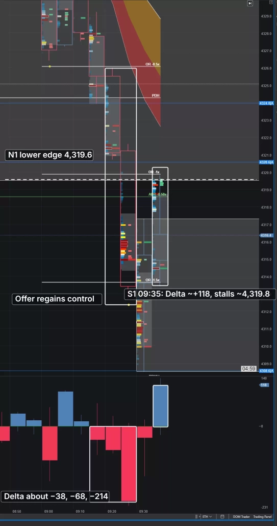
Figure 9 | Gold M5, September 25, 09:40 ET. After N1 was lost, retest S1 brought buying without sustained recovery. The 09:25 bar fell from about 4,321 to 4,314 (Delta near −214); S1 at 09:35 showed Delta +118 but stalled near 4,319.8.
The retracement toward the 4,320s was the test. Buying struggled to make any material gain while the offer regained effectiveness; Figure 10 shows the buyers who lifted the retest stalling beneath the zone marked Δ+83. A previously meaningful reference had changed its role, supporting my second agenda: a re-offer against offside inventory higher. I shorted the retracement (marker 1), with the stop at 4,319.9, just beyond those buyers. Sustained bid activity back above the node would have weakened the thesis.
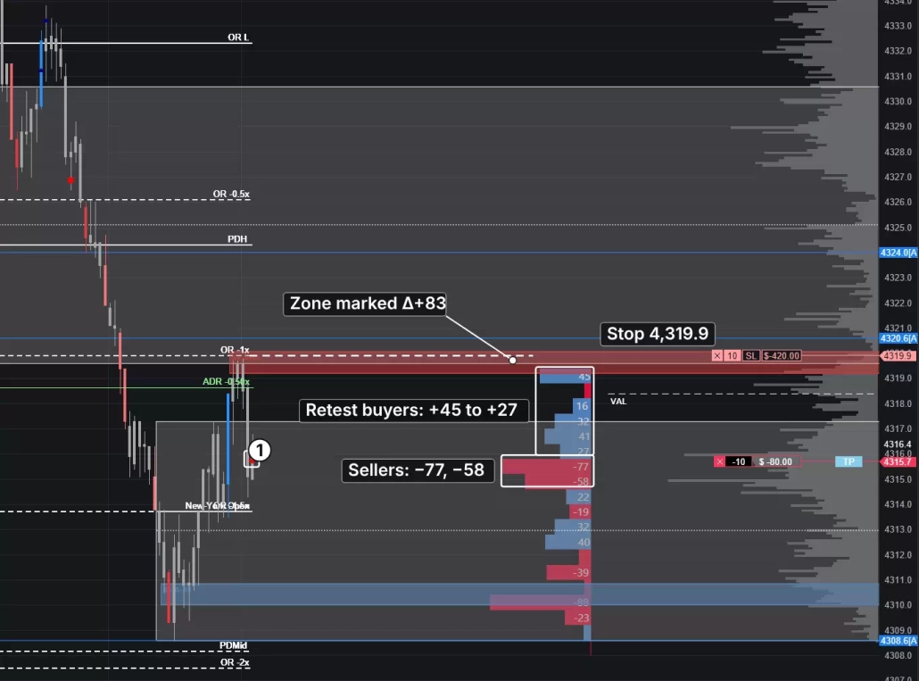
Figure 10 | Gold 150V, September 25, 09:40:05 ET. Retest buying stalls beneath Δ+83; marker 1 identifies short entries. Retest buyers about +45 to +27 between 4,316 and 4,319.4.
The offer continued to fill inventory lower, while the bid’s attempted reclaim near 4,318.6 was rejected, leaving earlier buying vulnerable before the liquidation pushed price through the range and into the low of the day. In Figure 11, the 10:00 bar displaced price through Thursday’s POC with heavy negative Delta, and the leg to leg delta profile shows the heaviest selling at 4,299 to 4,300. This time, aggressive selling produced displacement.
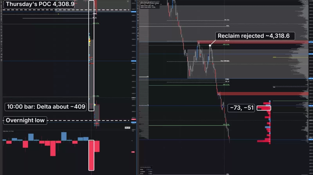
Figure 11 | Gold M5 and 150V, September 25, 10:05:28 ET. Lower discovery follows the failed recovery. The 10:00 bar is complete; the current bar is developing. The 10:00 bar ran from 4,310.7 to 4,293.3 with Delta near −409; the heaviest leg selling was about −73 and −51.
Although the sequence may appear flexible, it was the simplicity of following a predefined game plan that let me weigh specific activity at specific prices. The market did not owe my original long hypothesis a favorable result. The same process governed both decisions: establish what is known, define what remains unresolved, identify the response required, and change the interpretation when that response fails.
Common Mistakes When Trading Auction Market Theory
- Trying to know participants’ intentions. There are various tools that show us where aggressive transactions occurred, how much business was conducted, and whether that activity produced meaningful price progress, but never why. Our responsibility does not lie in needing to explain their intentions, but to interpret the footprint their activity leaves behind.
- Using every tool available. I made this mistake through several stages of my development: many traders execute through the Depth of Market (DOM), but for me its speed and volume of information overwhelmed my ability to read the tape. I am a firm believer in the 80/20 principle: a small minority of inputs often accounts for most of the meaningful output. Our objective should not be to see everything, but to identify the information that actually improves our decisions.
- Assuming more information means less uncertainty. Information is inherently incomplete, and two seemingly identical opportunities can produce entirely different outcomes. Waiting for more evidence also changes the price available and the distance to the next reference; confirmation has a cost, just as acting early does.
- Treating AMT as the edge. AMT is a methodology through which an edge can be identified and developed. An edge requires a mechanical and repeatable cause-and-effect relationship, with clearly defined conditions, and a risk model built around the possibility of being wrong.
The final note I will leave you with is that the objective is not to know what the market will do; there is no way of knowing. It is by recognizing the few conditions worth participating in, and those that are not, that we can apply our own positive and negative feedback loops to learn, adapt and improve.
Auction Market Theory Trading FAQ
Start with location. Establish what the higher timeframe has already decided using volume profile nodes and reference levels, define what remains unresolved, build if-then scenarios with clear invalidation, and then test those scenarios on the lower timeframe with Order Flow before committing risk.
Look for the point of control (POC), high volume nodes where the market built two-way trade and accepted price, and low volume nodes where price moved quickly with little trade. Combine them with market-generated references such as prior day and week highs and lows, opens and the initial balance.
Three outcomes can be told apart: efficient traversal, where price moves through quickly toward the next distribution; rejection, where the probe makes limited progress and price returns; and new acceptance, where fresh volume builds inside the thin area.
Compare effort with result. Volume and Delta show how much aggression occurred and which side initiated; price response shows whether that aggression produced progress. A large Delta bar that fails to extend often means the aggression was absorbed.
Daily, one-hour, five-minute footprint and 150-contract volume charts, volume profiles (Volume Profile & TPO or Fixed Volume Profile & TPO), the native Delta indicator and footprint settings that show volume by price. Custom studies speed up the work, but each one has a native ATAS route.
No. AMT is a methodology through which an edge can be identified and developed. An edge requires a repeatable cause-and-effect relationship, clearly defined conditions and a risk model built around the possibility of being wrong.
Information in this article cannot be perceived as a call for investing or buying/selling of any asset on the exchange. All situations, discussed in the article, are provided with the purpose of getting acquainted with the functionality and advantages of the ATAS platform.
Subscribe
Get the latest ATAS news delivered conveniently